After part one which covered an overview of Keras and PyTorch syntaxes, this is part two of how to switch between Keras and PyTorch. We will implement a neural network to classify movie reviews by sentiment.
- Keras is aimed at fast prototyping. It is designed to write less code, letting the developper focus on other tasks such as data preparation, processing, cleaning, etc
- PyTorch is aimed at modularity and versatility. Fine-grained control on the flow of computations
Yet both frameworks are meant to do the same, that is training deep neural networks. The number of resources of "rosetta stone" style tutorials is very limited on internet, especially resources demonstrating practical examples, so I hope this will help demistifying the differences and similarities between the two frameworks. Now let's get started!
Dataset of IMDB movie reviews
We will use IMDB dataset, a popular toy dataset in machine learning, which consists of movie reviews from the IMDB website annotated by positive or negative sentiment.
Both Keras and PyTorch have helper functions to download and load the IMDB dataset. So instead of using dataloaders as we saw in part one we will use this code in which we import the IMDB dataset in Keras.
from tensorflow.keras.datasets import imdb
input_dim = 20000
(x_train, y_train), (x_val, y_val) = imdb.load_data(num_words=input_dim)
print(len(x_train), "Training sequences")
print(len(x_val), "Validation sequences")
This creates a data/ folder and downloads the dataset inside. It splits the data in half into training and validation sets. The output gives the number of sequences
25000 Training sequences
25000 Validation sequences
With torchtext, PyTorch can also download and load the IMDB dataset in the same fashion. Yet, to make sure the data we feed to Keras and the data we feed to PyTorch is the same, I will simply adapt the downloaded data using Keras to PyTorch, so we are sure to have consistency between both implementations, especially in terms of data cleaning and how the text is tokenized.
In addition, we will pad the movie reviews to have sequences of same length. This is important to train on batches as it is not possible to parallelize computation of the error gradient on sequences of variable length.
from tensorflow.keras.preprocessing.sequence import pad_sequences
maxlen = 200
x_train = pad_sequences(x_train, maxlen=maxlen)
x_val = pad_sequences(x_val, maxlen=maxlen)
We fix the length of reviews to 200 word tokens and the vocabulary to 20k different word tokens. The dataset is already cleaned and tokenized so we can directly feed it to the neural networks! Before proceeding, We may take a look at some examples in our dataset out of curiosity. We need to get the word vocabulary using imdb.get_word_index which will let us decode that bunch of integers from the dataset into plain english.
index_offset = 3
word_index = imdb.get_word_index(path="imdb_word_index.json")
word_index = {k: (v + index_offset) for k,v in word_index.items()}
word_index["<PAD>"] = 0
word_index["<START>"] = 1
word_index["<UNK>"] = 2
word_index["<UNUSED>"] = 3
index_to_word = { v: k for k, v in word_index.items()}

def recover_text(sample, index_to_word):
 return ' '.join([index_to_word[i] for i in sample])

recover_text(x_train[50], index_to_word)
With the above code we can check that the sequence 1, 13, 165, 219, 14, 20, 33, 6, 750, ... from the dataset corresponds to
<START> i actually saw this movie at a theater as soon as i handed the cashier my money she said two words i had never heard at a theater before or since no <UNK> as soon as i heard those words i should have just <UNK> bye bye to my cash and gone home but no foolishly i went in and watched the movie this movie didn't make anyone in the theater laugh not even once not even <UNK> mostly we sat there in stunned silence every ten minutes or so someone would yell this movie sucks the audience would applaud enthusiastically then sit there in stunned bored silence for another ten minutes <PAD> <PAD> <PAD> […]
We can print the sentiment associated with this review, it is y_train[50] which is 0 for "negative". Looks right.
But wait! We need to adapt our data for PyTorch. This code will do the job.
from torch.utils.data import TensorDataset, DataLoader
train_data = TensorDataset(torch.from_numpy(x_train), torch.from_numpy(y_train))
valid_data = TensorDataset(torch.from_numpy(x_val), torch.from_numpy(y_val))
train_loader = DataLoader(train_data, shuffle=True, batch_size=batch_size, drop_last=True)
valid_loader = DataLoader(valid_data, shuffle=True, batch_size=batch_size, drop_last=True)
The TensorDataset class will convert our data to torch tensors, slice into batches, and shuffle. Then with a DataLoader instance we will be able to iterate over the batches.
A side note here, concerning the use of DataLoader instance to load the data. It seems to guarantee some numerical stability during training, because my experimentations demonstrated that when manually shuffling and slicing the data from the train_data and valid_data tensors gave poor classification results, the model being unable to effectively train.
Good! The data is ready, let's define our classifiers.
Classifier model
Our classifier is a bidirectional two-layers LSTM on top of an embedding layer, and followed by a dense layer which gives one output value. This output value gives the probability of a review being positive. the closer to zero, the more negative the review is predicted and the closer to one, the more positive the review is predicted. To obtain such probability, we use a sigmoid function, which takes the final output of the neural network and squeezes the value between 0 and 1.
We will define the two following hyperparameters to make sure both implementations match.
embedding_dim = 128
hidden_dim = 64
Let's start with Keras (credits to the official Keras documentation1.)
from tensorflow.keras.layers import Bidirectional, LSTM, Dense, Embedding
from tensorflow.keras.models import Sequential
model = Sequential([
  Embedding(input_dim, 128),
  Bidirectional(LSTM(hidden_dim, return_sequences=True)),
  Bidirectional(LSTM(hidden_dim)),
  Dense(1, activation="sigmoid")
])
model.compile(optimizer='adam', loss='binary_crossentropy', metrics=["accuracy"])
model.summary()
Now, let's implement the same in PyTorch. Hang in there, because there are some technical subtelties to be aware of. I want to show you first what would be a naive implementation
import torch
from torch import nn
class BiLSTM(nn.Module):
  def __init__(self, input_dim, embedding_dim, hidden_dim):
      super().__init__()
      self.input_dim = input_dim
      self.embedding_dim = embedding_dim
      self.hidden_dim = hidden_dim
      self.encoder = nn.Embedding(input_dim, embedding_dim)
      self.lstm = nn.LSTM(embedding_dim, hidden_dim,
                          num_layers=2, bidirectional=True)
      self.linear = nn.Linear(hidden_dim * 2, 1)
      self.activation = nn.Sigmoid()

  def forward(self, src):
      batch_size = src.size(1)
      output = self.encoder(src)
      output, _ = self.lstm(output)
       output = self.linear(output)
      output = self.activation(output)
      return output
If you read part one, there won't be any surprise in this code. In PyTorch we simply detail a bit more the computation whereas Keras infer them as we stack the layers.
Now the sad news is this implementation is not exactly the same as the one with Keras. And the main difference is initialization! It requires a fair amount of digging to make both frameworks agree on initializations. For example, you can see that the Embedding layer from Keras initialize its weights with a uniform distribution, whereas it is a normal distribution which is used by PyTorch. Let's get straight to the point and use the following method to adapt PyTorch initialization to Keras.
def init_weights(self):
  self.encoder.weight.data.uniform_(-0.5, 0.5)
  ih = (param.data for name, param in self.named_parameters() if 'weight_ih' in name)
  hh = (param.data for name, param in self.named_parameters() if 'weight_hh' in name)
  b = (param.data for name, param in self.named_parameters() if 'bias' in name)
  for t in ih:
      nn.init.xavier_uniform(t)
  for t in hh:
      nn.init.orthogonal(t)
  for t in b:
      nn.init.constant(t, 0)
It is a nice snippet taken from torchMoji, a PyTorch implementation of DeepMoji by HuggingFace. We now have our updated BiLSTM class in PyTorch
import torch
from torch import nn
class BiLSTM(nn.Module):
  def __init__(self, input_dim, embedding_dim, hidden_dim):
      super().__init__()
      self.input_dim = input_dim
      self.embedding_dim = embedding_dim
      self.hidden_dim = hidden_dim
      self.encoder = nn.Embedding(input_dim, embedding_dim)
      self.lstm = nn.LSTM(embedding_dim, hidden_dim,
                          num_layers=2, bidirectional=True)
      self.linear = nn.Linear(hidden_dim * 2, 1)
      self.activation = nn.Sigmoid()

      nn.init.xavier_uniform_(self.linear.weight)
      self.linear.bias.data.zero_()
      self.init_weights()

  def init_weights(self):
      ih = (param.data for name, param in self.named_parameters() if 'weight_ih' in name)
      hh = (param.data for name, param in self.named_parameters() if 'weight_hh' in name)
      b = (param.data for name, param in self.named_parameters() if 'bias' in name)
      self.encoder.weight.data.uniform_(-0.5, 0.5)
      for t in ih:
          nn.init.xavier_uniform(t)
      for t in hh:
          nn.init.orthogonal(t)
      for t in b:
          nn.init.constant(t, 0)

  def forward(self, src):
      batch_size = src.size(1)
      output = self.encoder(src)
      output, _ = self.lstm(output)
      output = nn.functional.tanh(output[-1])
      output = self.linear(output)
      output = self.activation(output)
      return output, None
Well… As you can see, even for very basic architectures, transferring code is not an easy job. And even the details are quite important to achieve similar results, but bear with me, because this is the closest I could get to the Keras implementation.
A quick sanity check would be to verify the number of parameters of both implementations match. model.summary() in Keras outputs the following.
 Model: "sequential"
_________________________________________________________________
Layer (type)                 Output Shape              Param #
=================================================================
embedding (Embedding)        (None, None, 128)         2560000
_________________________________________________________________
bidirectional (Bidirectional (None, None, 128)         98816
_________________________________________________________________
bidirectional_1 (Bidirection (None, 128)               98816
_________________________________________________________________
dense (Dense)                (None, 1)                 129
=================================================================
Total params: 2,757,761
Trainable params: 2,757,761
Non-trainable params: 0
_________________________________________________________________
Printing the model in PyTorch with print(model) shows we have the same architecture.
BiLSTM(
(encoder): Embedding(20000, 128)
(lstm): LSTM(128, 64, num_layers=2, bidirectional=True)
(linear): Linear(in_features=128, out_features=1, bias=True)
(activation): Sigmoid()
)
But this does not inform us on the number of parameters. This line gives what we want (thanks to Federico Baldassare)
sum(p.numel() for p in model.parameters() if p.requires_grad)This gives 2758785 parameters. Oh! The numbers of parameters are different!? After digging this issue, I found out PyTorch has a second bias tensor for compatibility reasons with CuDNN in its implementation of the LSTM. You can effectively check that the count difference is equal to 2,758,785 - 2,757,761 = 1024, which is 2 * 4 * 2 * 64 = 1024. where we multiply 64, the size of the bias vector of one LSTM cell by 2, because we have a forward and a backward LSTM, 2 again because we use two layers, and 4 which is the number of gates in the definition of the LSTM. Even with a basic architecture like this one, subtle yet important differences arise.
Now let's check how the implementations perform.
Training
We will use the following parameters for training.
batch_size=32
epochs = 2
In Keras, this one line will do
model.fit(x=x_train, y=y_train,
        batch_size=batch_size, epochs=epochs,
        validation_data=(x_val, y_val))
Now with PyTorch, remember that everything Keras does under the hood must be explicitly written. First is to initialize the logs, loss criterion, model, device and optimizer.
model = BiLSTM(input_dim, embedding_dim, hidden_dim)
device = torch.device("cuda" if torch.cuda.is_available() else "cpu")
criterion = nn.BCELoss().to(device)
optimizer = torch.optim.Adam(model.parameters())
model.to(device)
batch_history = {
    "loss": [],
    "accuracy": []
}
epoch_history = {
    "loss": [],
    "accuracy": [],
    "val_loss": [],
    "val_accuracy": [],
}
What follows is the training loop. I use the tqdm library which I recommend for printing a nice progress bar in the same fashion as Keras.
from tqdm import tqdm, trange
for i in trange(epochs, unit="epoch", desc="Train"):
    model.train()
    with tqdm(train_loader, desc="Train") as tbatch:
        for i, (samples, targets) in enumerate(tbatch):
            model.train()
            samples = samples.to(device).long()
            targets = targets.to(device)
            model.zero_grad()
            predictions, _ = model(samples.transpose(0, 1))
            loss = criterion(predictions.squeeze(), targets.float())
            acc = (predictions.round().squeeze() == targets).sum().item()
            acc = acc / batch_size
            loss.backward()
            torch.nn.utils.clip_grad_norm_(model.parameters(), 5)
            optimizer.step()

            batch_history["loss"].append(loss.item())
            batch_history["accuracy"].append(acc)

            tbatch.set_postfix(loss=sum(batch_history["loss"]) / len(batch_history["loss"]),
                               acc=sum(batch_history["accuracy"]) / len(batch_history["accuracy"]))
Notice the use of model.train() and model.eval() methods which set model.training to either True or False. It decides whether or not to keep the gradient during the forward pass, which will be used for optimizing the network in the backward pass.
I used torch.nn.utils.clip_grad_norm_(model.parameters(), 5) to clip weight gradients to 5. I am not sure how Keras deals with gradient clipping but it is usually good practice to implement this technique to avoid the problem of exploding gradient.
A final remark concerns the ordering of dimensions. As I explained in part one, Keras expects by default batch dimension to be first while PyTorch expects it in second position. So with samples.transpose(0, 1) we effectively permute first and second dimensions to fit PyTorch data model.
Now, likewise Keras, when we reach the end of an epoch, we want to evaluate the model.
epoch_history["loss"].append(sum(batch_history["loss"]) / len(batch_history["loss"]))
epoch_history["accuracy"].append(sum(batch_history["accuracy"]) / len(batch_history["accuracy"]))
model.eval()
print("Validation...")
val_loss, val_accuracy = validate(model, valid_loader)
epoch_history["val_loss"].append(val_loss)
epoch_history["val_accuracy"].append(val_accuracy)
print(f"{epoch_history=}")
Results
In the following tables I report results for each training epoch, averaged over the number of batches.
| Epoch | loss (Keras) | loss (PyTorch) | accuracy (Keras) | accuracy (PyTorch) |
|---|---|---|---|---|
| 1 | 0.4479 | 0.4881 | 0.7916 | 0.7556 |
| 2 | 0.2855 | 0.3962 | 0.8880 | 0.8173 |
| Epoch | val_loss (Keras) | val_loss (PyTorch) | val_accuracy (Keras) | val_accuracy (PyTorch) |
|---|---|---|---|---|
| 1 | 0.3639 | 0.4024 | 0.8440 | 0.8233 |
| 2 | 0.3468 | 0.3343 | 0.8542 | 0.8624 |
The following graphs show the loss and binary accuracy on batch during training.
Batch training loss Batch training accuracy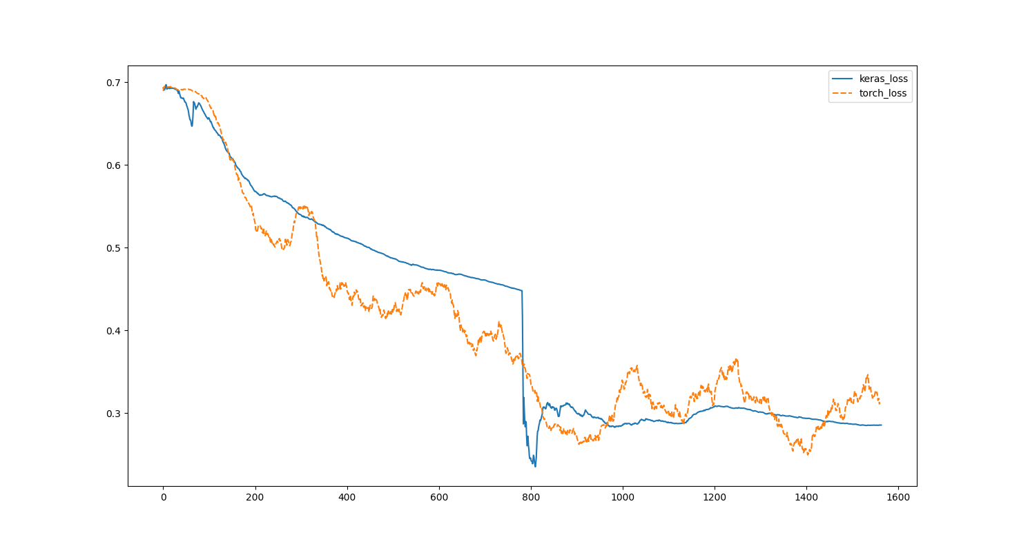
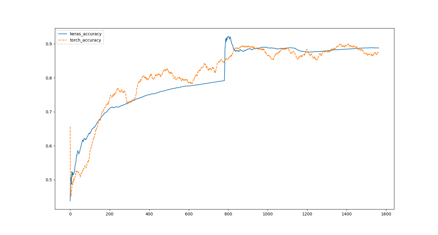
We can notice a sudden jump in accuracy and loss for the Keras implementation. This may be reduced if we optimize the learning rate.
Last words
Even with great care, it is hard to obtain the very same results with identical architecture, data processing and training, because each framework has its own internal mechanisms, designs, with in addition specific tricks to guarantee numerical stability. Nonetheless, the results we got are close.
There are ambitious projects such as ONNX creating a standard between deep learning frameworks, to practically solve the discrepancies we witnessed in this article.
I hope you enjoyed this comparison of Keras and PyTorch want to read your ideas and feedbacks! Hope you the best in your machine learning journey!